

Best Color Palettes for Graphics Statistics in R
Using a Different Palette for a Discrete Variable
Problem
You want to use different colors for a discrete mapped variable.
Solution
Use one of the scales listed in Table 12.1.
| Fill scale | Color scale | Description |
|---|---|---|
scale_fill_discrete() | scale_colour_discrete() | Colors evenly spaced around the color wheel (same as hue) |
scale_fill_hue() | scale_colour_hue() | Colors evenly spaced around the color wheel (same as discrete) |
scale_fill_grey() | scale_colour_grey() | Greyscale palette |
scale_fill_viridis_d() | scale_colour_viridis_d() | Viridis palettes |
scale_fill_brewer() | scale_colour_brewer() | ColorBrewer palettes |
scale_fill_manual() | scale_colour_manual() | Manually specified colors |
In the example here we'll use the default palette (hue), a viridis palette, and a ColorBrewer palette (Figure 12.6):
library(gcookbook) # Load gcookbook for the uspopage data set library(viridis) # Load viridis for the viridis palette # Create the base plot uspopage_plot <- ggplot(uspopage, aes(x = Year, y = Thousands, fill = AgeGroup)) + geom_area() # These four specifications all have the same effect uspopage_plot # uspopage_plot + scale_fill_discrete() # uspopage_plot + scale_fill_hue() # uspopage_plot + scale_color_viridis() # Viridis palette uspopage_plot + scale_fill_viridis(discrete = TRUE) # ColorBrewer palette uspopage_plot + scale_fill_brewer() 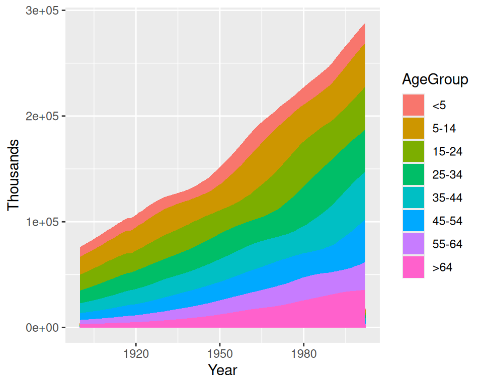
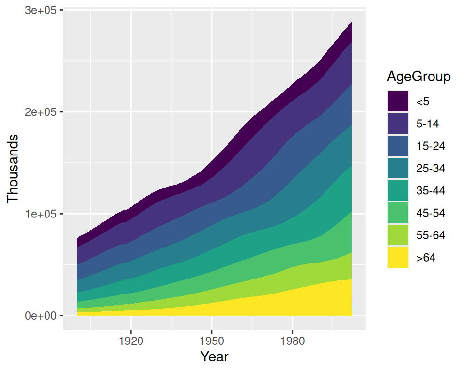
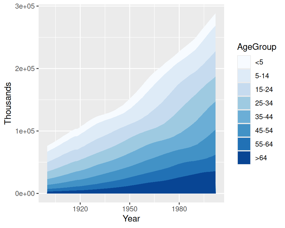
Figure 12.6: Default palette (using hue; top); A viridis palette (middle); A ColorBrewer palette (bottom)
Discussion
Changing a palette is a modification of the color (or fill) scale: it involves a change in the mapping from numeric or categorical values to aesthetic attributes. There are two types of scales that use colors: fill scales and color scales.
With scale_fill_hue(), the colors are taken from around the color wheel in the HCL (hue-chroma-lightness) color space. The default lightness value is 65 on a scale from 0–100. This is good for filled areas, but it's a bit light for points and lines. To make the colors darker for points and lines, as in Figure 12.7 (right), set the value of l (luminance/lightness):
# Create the base scatter plot hw_splot <- ggplot(heightweight, aes(x = ageYear, y = heightIn, colour = sex)) + geom_point() # Default lightness = 65 hw_splot # Slightly darker, set lightness = 45 hw_splot + scale_colour_hue(l = 45) 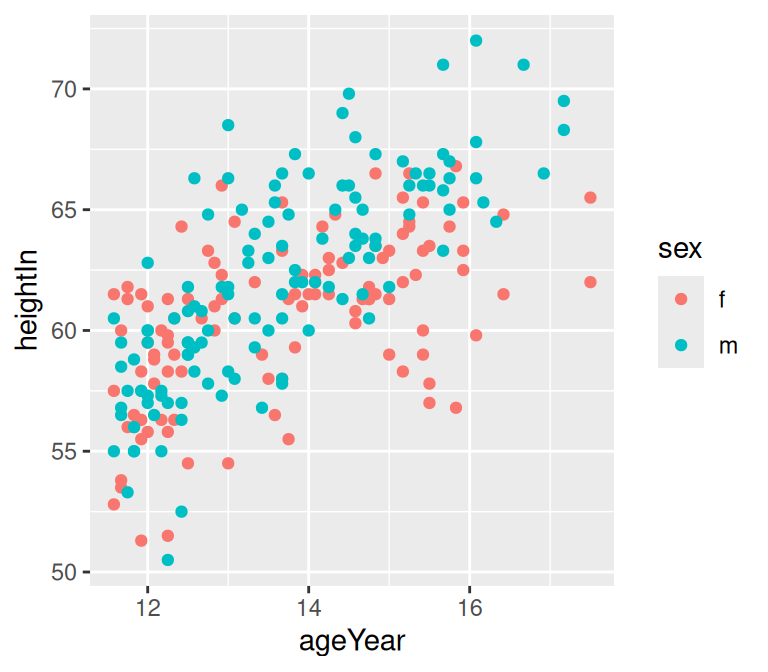
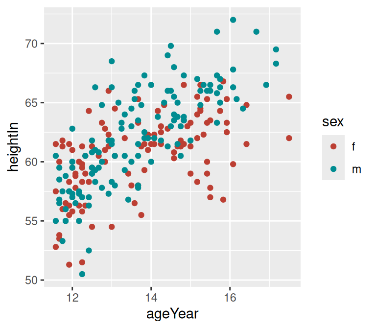
Figure 12.7: Points with default lightness (left); With lightness set to 45 (right)
The viridis package provides a number of color scales that make it easy to see differences across your data. See Recipe 12.3 for more details and examples.
The ColorBrewer package provides a number of palettes. You can generate a graphic showing all of them, as shown in Figure 12.8:
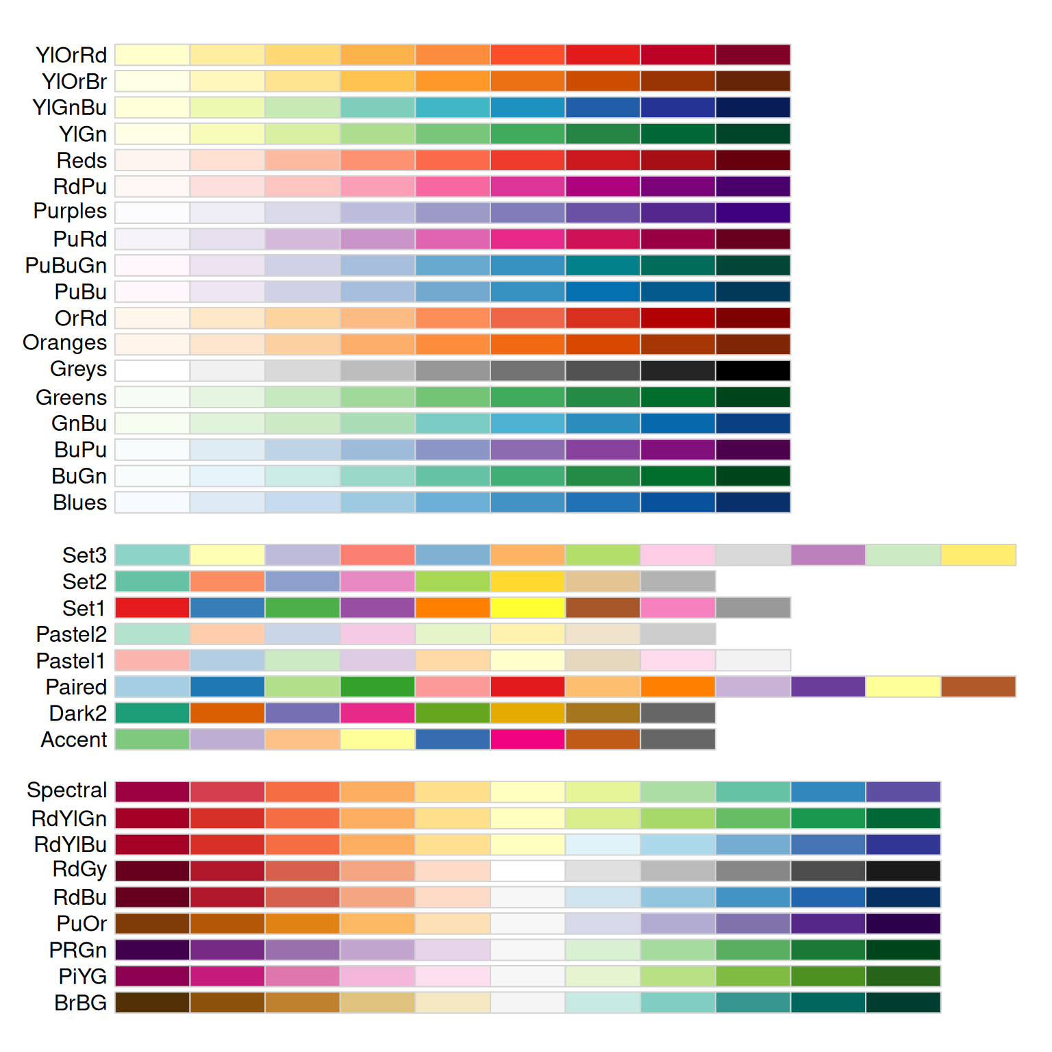
Figure 12.8: All the ColorBrewer palettes
library(RColorBrewer) display.brewer.all() The ColorBrewer palettes can be selected by name. For example, this will use the "Oranges" palette (Figure 12.9):
hw_splot + scale_colour_brewer(palette = "Oranges") + theme_bw() 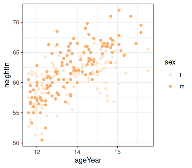
Figure 12.9: Using a named ColorBrewer palette
You can also use a palette of greys. This is useful for print when the output is in black and white. The default is to start at 0.2 and end at 0.8, on a scale from 0 (black) to 1 (white), but you can change the range, as shown in Figure 12.10.
hw_splot + scale_colour_grey() # Reverse the direction and use a different range of greys hw_splot + scale_colour_grey(start = 0.7, end = 0) 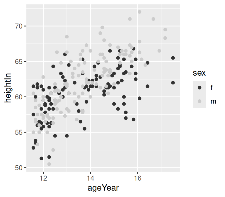
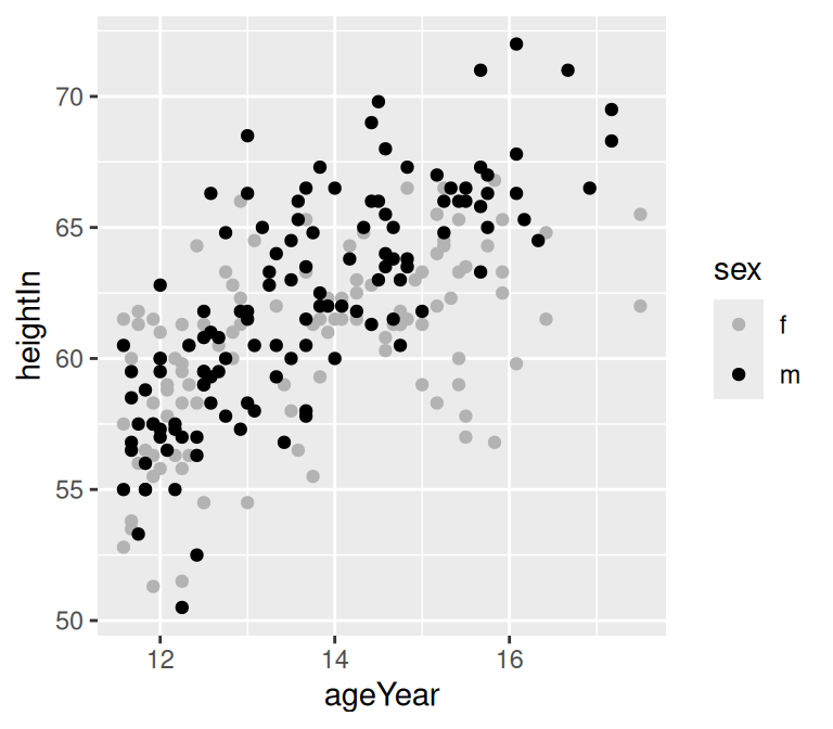
Figure 12.10: Using the default grey palette (left); A different grey palette (right)
Best Color Palettes for Graphics Statistics in R
Source: https://r-graphics.org/recipe-colors-palette-discrete
0 Response to "Best Color Palettes for Graphics Statistics in R"
Post a Comment